In this article, I will be doing a deeper analysis of Quick Sort, and how by using the concept of probability, we are able to optimise its sorting algorithm. This article assumes knowledge of the usage of arrays (in C++), and more importantly, knowledge of Quick Sort. If not, do check out my article here.
Concept of ‘Boundary Pivots’
Before I begin on the analysis, I would first be explaining what a boundary pivot is. A boundary pivot is a chosen pivot (by the Quick Sort algorithm) that lies at the edge of the array. This means that its index is either less than N/10 or greater than 9N/10 (smallest 10% or largest 10%). In the extreme cases, we would have an already sorted array, which is why I previously stated that Quick Sort has O(N^2) Time Complexity in those cases.

In this case, the given array is already in sorted in ascending order. When we perform Quick Sort by taking the first element as the pivot, our left pointer, i, moves up one index, and waits for the right pointer, j, to find an element smaller than or equal to the pivot element. When the j eventually reaches that element, its index is less than the i’s, signifying the array has been traversed. As such, no swap is done, but N comparisons are done while traversing the array. Indeed, the pivot element is already in its correct spot, and the algorithm moves on to perform Quick Sort on the remaining elements.
For the entire sorting algorithm, it would be evaluated that in the first round, N comparisons are done, and in the second round, (N-1) comparisons are done, and so on, until the last round, where 1 comparison is done. By summing everything up, we will get a time complexity of O((N(N+1))/2), which is O(N^2).
How to pivot well
Based on the previous part, we have established the importance of choosing a good pivot. Now, the question lies in how we choose our pivots, to ensure that they are good. As demonstrated in the height swapping example, we can see that, if we were to perfectly bisect the array with our pivot, less work would be done in pivoting every element. An illustration of this is show below, but keep in mind that the illustration shown is an extreme case.
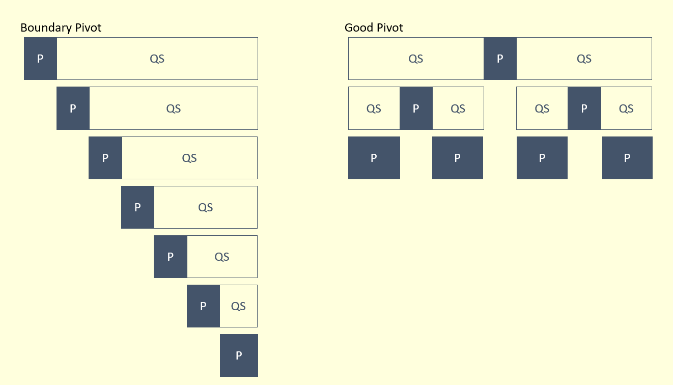
In order to perfectly bisect our array with our pivot, we would have to always choose the median of the array to be the pivot. But if the array was unsorted, how do we do this? Fortunately, there is actually no need to choose the median! For the sake of this article, I will define boundary elements as indexes less than N/10 or greater than 9N/10, which corresponds to the smallest and largest 10% respectively. A good pivot is definitely not a boundary element, and thus, it will cut the array minimally into a 1:9 ratio.
 As the diagram displays, even if a 1:9 ratio pivot was done, it will still be optimal, and achieve a time complexity of O(N log N). Therefore, we have actually proven that there is no need to perfectly bisect an array by finding and pivoting its median.
In this case, the next question would then be, how do we obtain this good pivot?
Probability Analysis of Random Pivots
 Since we are trying to avoid the boundary pivots (bottom and top 10%), that means that we are able to select 80% of the elements as pivots, and they will be good pivots. As such, the probability of selecting a good pivot will be 80%, or 0.8. With this knowledge, the expected number of partitions required to obtain a good pivot would be the inverse of the probability, which would give us 1/0.8 = 1.25. With this knowledge, we can safely expect there to be one good pivot, in every 2 partitions, which means we will only repeat the partition O(1) times!
With this knowledge, we can now use probability to check and improve on our Quick Sort Partitioning algorithm.
Improved Partitioning Algorithm
// Expected number of partitions needed: 2
int randomPartition(int* arr, int low, int high) {
  int n = high-low;
  int random = low + rand()%n;
  swap(arr[low], arr[random]);
  int rp = partition(arr, low, high);
  // n <= 1 implies 1 or 2 elements
  // No need for repartition
  if (n > 2 && (rp < n/10.0 || rp > 9*n/10.0)) {
    random = low + rand()%n;
    swap(arr[low], arr[random]);
    rp = partition(arr, low, high);
  }
  return rp;
}
Conclusion
We have just taken a look at how the Quick Sort algorithm can be improved by allowing it to make decisions based on randomness. However, we have also seen that we can have a good chance of success, by analysing the probability and expected outcome of our algorithm. With this implementation, we can now say that Randomised Quick Sort always has a time complexity of O(N log N).